
Self-Supervised Learning & Wav2Vec 2.0

Different machine learning training techniques are appropriate based on the data availability:
Supervised: all our data is labelled.
Semi-supervised: a small amount of our data is labelled.
Unsupervised: none of our data is labelled.
Self-supervised: none of our data is labelled.
In this blog we will be looking at self-supervised learning techniques to create representations of audio waveforms.
Audio data captured from a microphone is inherently difficult to work with for many applications because waveforms have a high temporal dimensionality and poor structure. An ideal representation of audio would have low dimensionality and structure from which it is easy to learn downstream tasks.
Mel Spectrograms
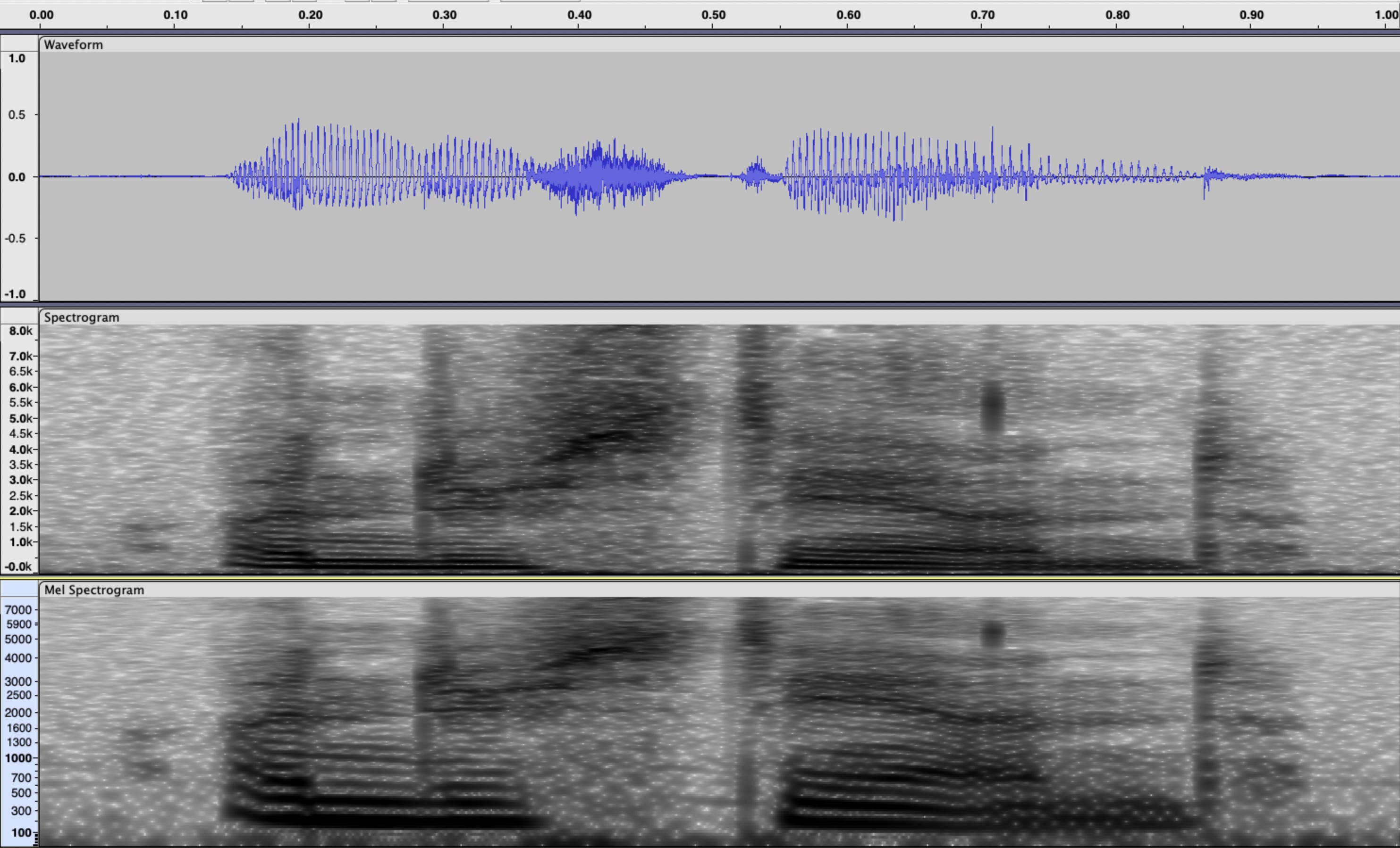
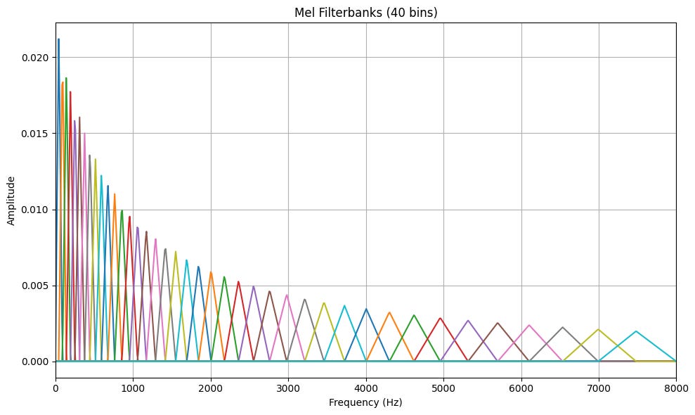
One alternative to waveform data is to use the short time Fourier transform (STFT) to generate a spectrogram of our audio data. This representation is typically more useful, as the time-frequency structure reflects human perception of sound. The STFT still has a high dimensionality, so we can apply a mel filterbank to average magnitude frequency bins, based on heuristics derived from human hearing. This reduces the dimensionality, but we are discarding information because of the bin-averaging.
Wav2Vec 2.0
An alternative to the mel spectrogram is to use Wav2Vec 2.0 to generate self-supervised representations of audio data. At a high level, Wav2Vec 2.0 asks if we can find a ‘better’ transformation of the audio waveform into features. Better in this sense means that we can achieve better performance on downstream tasks, such as automatic speech recognition, than if we had used the mel spectrogram.
Although this post explores self-supervised learning from the perspective of audio, it is a technique that is widely used in machine learning, especially for large language models in which we would seek to learn interesting representations of words.
Network Architecture
First I will describe the network architecture as it would be initialized prior to training. At initialization time, we can think of all the layers in Wav2Vec 2.0 as performing random mapping, from one representation to another. Later, we will show how we can set up an objective function to teach our neural networks ‘interesting’ mappings that lead to ‘good’ representations.
Feature Encoder & Latent Speech Representations
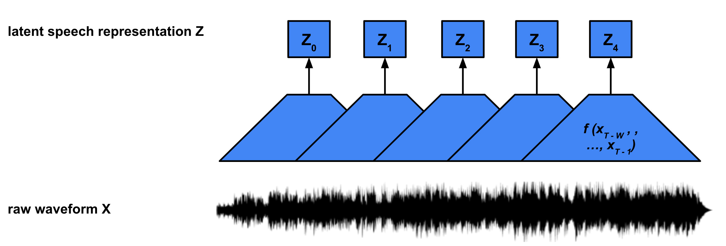
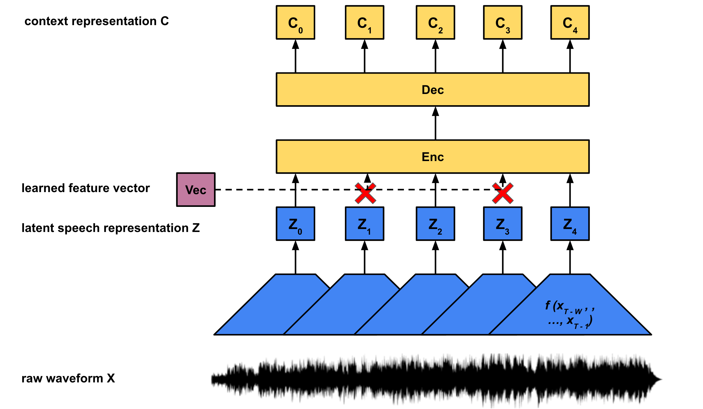
The feature encoder is a convolutional neural network (CNN) that maps a window of audio samples (X) to a learned latent (Z) vector, f : X → Z. The CNN has a fixed window size w and moves over the input audio with a hop size h. If our input audio utterance has T total samples, f (x0 , … , xw-1) maps to z0, f (xh , …, xw + h - 1) maps to z1, up until f (xT - w , … , xT - 1) maps to zN. Note the feature encoder will reduce the temporal dimensionality from T to approximately T / h, depending on how beginning and end of sequence padding is handled.
Masked Transformer & Context Representations
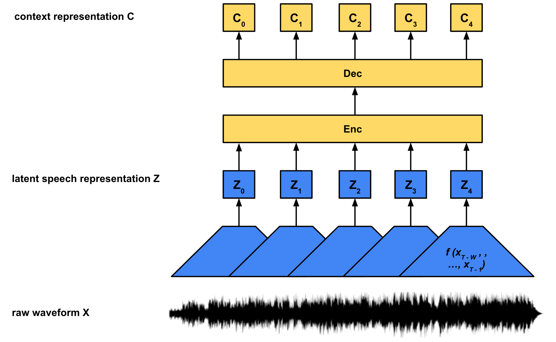
While each latent speech representation Z corresponds to a fixed block of length w of audio samples, X, the context representations C contain additional information about the entire utterance (that is all T samples in X). Rather than construct these context representations directly from the audio X, we construct them from the latent speech representations Z, g : Z → C. Wav2Vec 2.0 uses the transformer architecture from the seminal “Attention Is All You Need” paper to generate the context embeddings.
Masking
For each utterance, a certain proportion of inputs to the encoder are masked. Rather than masking by multiplying with an all 0 valued vector as is often done in the literature, the ‘masked’ latent speech representations are all replaced with one trained feature vector:
In the paper the authors chose an overall proportion p of latent vectors to start masking and also mask the subsequent M latent vectors.For an utterance with N latent vectors, N * p vectors are chosen as start indices. Since each mask covers M vectors, the masked spans can overlap. This means the total number of unique masked vectors will be less than or equal to N * p * M. This masking is used for the contrastive loss which we will discuss later.
Quantized Representations
The next problem we face is that the range of values for our Z are almost unbounded. For example, if our Z was a scalar and was stored with a standard IEEE float, our network could ‘cheat’ and learn to map one latent vector to one float value (or range of floats). For example, f(x0 , …, xw - 1) —> float(0b00000000000000000000000000000001), f(xh , …, xh + w - 1) —> float(0b00000000000000000000000000000010), etc. Although the network f is unlikely to learn this mapping in practice, it illustrates how the model could theoretically maintain a near lossless representation of the input audio. This defeats the purpose of forcing the model to group related segments of sound into a shared set of abstract speech units, which is the interesting latent representation we seek.
One solution is to use quantization to constrain the latent space. Let’s assume our latent vector Z has 2 dimensions, and we observed our CNN f map audio to the following vectors across out dataset:
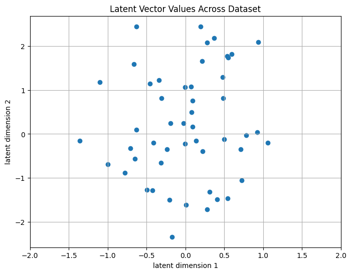
We want to restrict the values our latent vector can take. We can achieve this via unsupervised learning method such as k-means clustering to find centroids for our data. In k-means, we pre-select a number of centroids, and then estimate the coordinates that minimize the average distance to our data. Now, instead of our latent vector being able to take on an almost infinite range, we map each of the blue dots to the closest red dot:
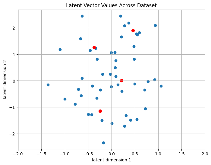
We now have a lossy representation of the entire dataset of 50 examples using only 2 bits, because we have 4 centroids (log2 4 = 2). We introduce quantization noise to our latent vectors, so we are losing information about them. However it forces the model to group similar latent vectors together. For example, latents representing audio with similar spectral envelopes may now map to the same centroid, instead of having different floating point representations.
Codevectors and Codebooks
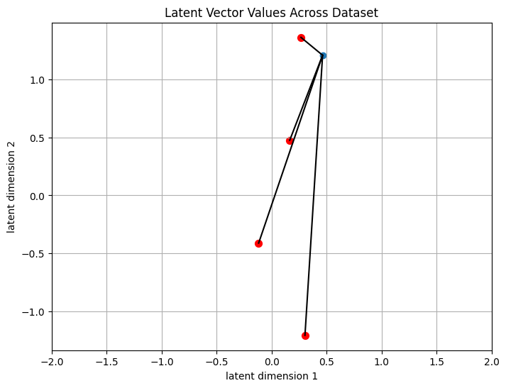
To encode a latent vector using our quantization scheme we need to find the nearest centroid for that vector. We call the nearest centroid to our latent vector the codevector. We can calculate the l2 distance between a candidate centroid and the latent vector we want to encode:
Where d is the dimensionality of our latent vector and centroids. We perform this comparison against every centroid and find the min.
The complexity of this algorithm grows as we increase both the dimensionality of our latent and the number of centroids. Wav2Vec 2.0 uses a latent vector dimensionality d of 256. We would need many codevectors to cover the space of latent vectors in a way that allows meaningful representations. In the paper, the authors use around 100,000 centroids. Naively, that would mean we need to do 256 x 100,000 = 25,600,000 subtraction operations to find the nearest codevector per latent vector. In reality this is too many operations to be computationally feasible both at inference and for training our quantizer.
Quantized Representations
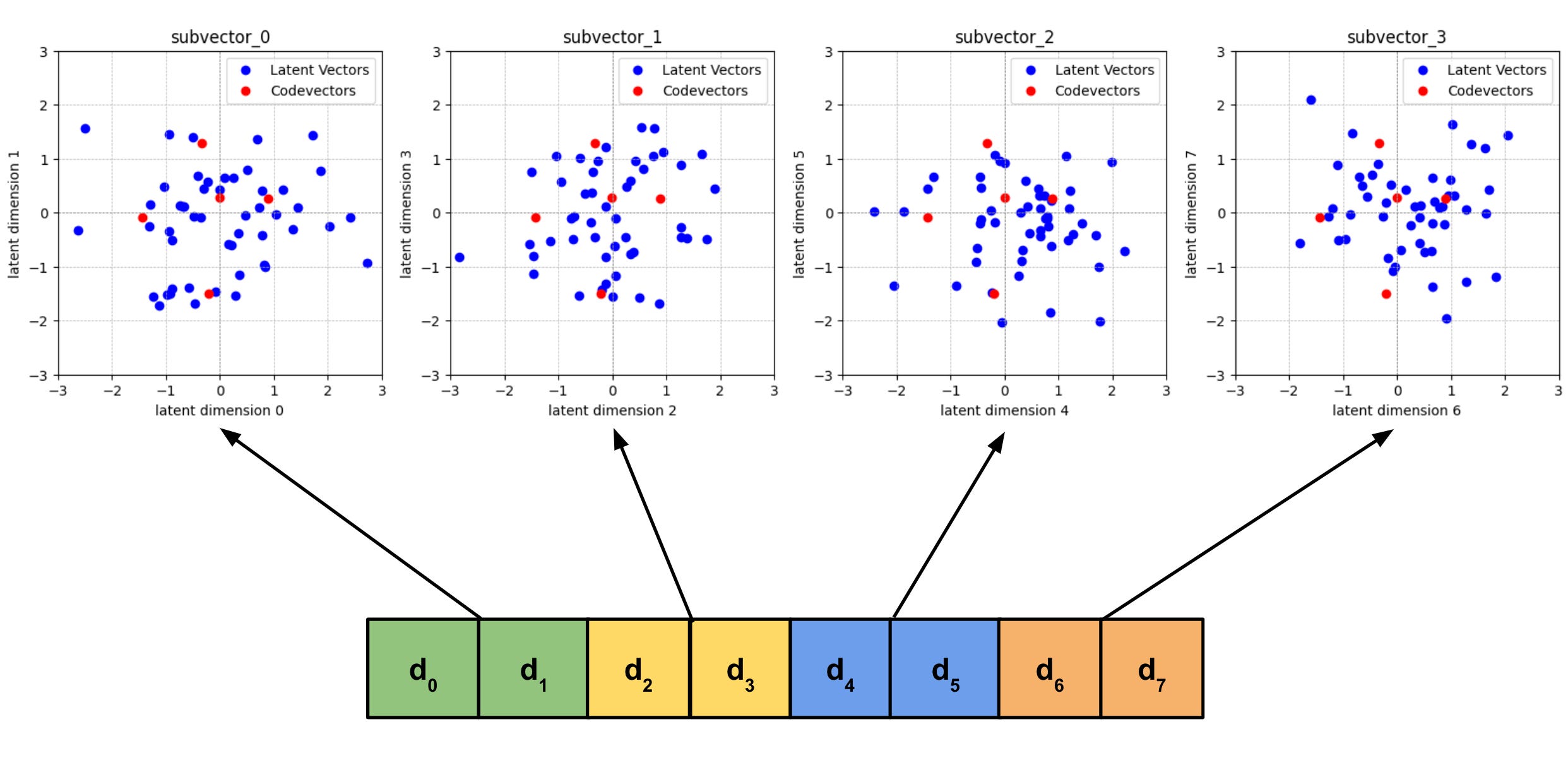
The authors instead use product quantization. In product quantization we split our latent vector into G subvectors of length equal to d / G, and quantize them separately. The set of codevectors we train for each subvector are called codebooks. We pick V codevectors per codebook. In the paper the authors chose V = 320 and G = 2. Given d = 256, we now need to do only G * (d / G) * V = 2 * 128 * 320 = 81,920 subtraction operations per latent vector, as opposed to 25,600,000. However with this setup we have a theoretical maximum of 320 * 320 = 102,400 codevectors. Using more codebooks and less codevectors per codebook allows us to decrease algorithmic complexity at the cost of adding quantization noise.
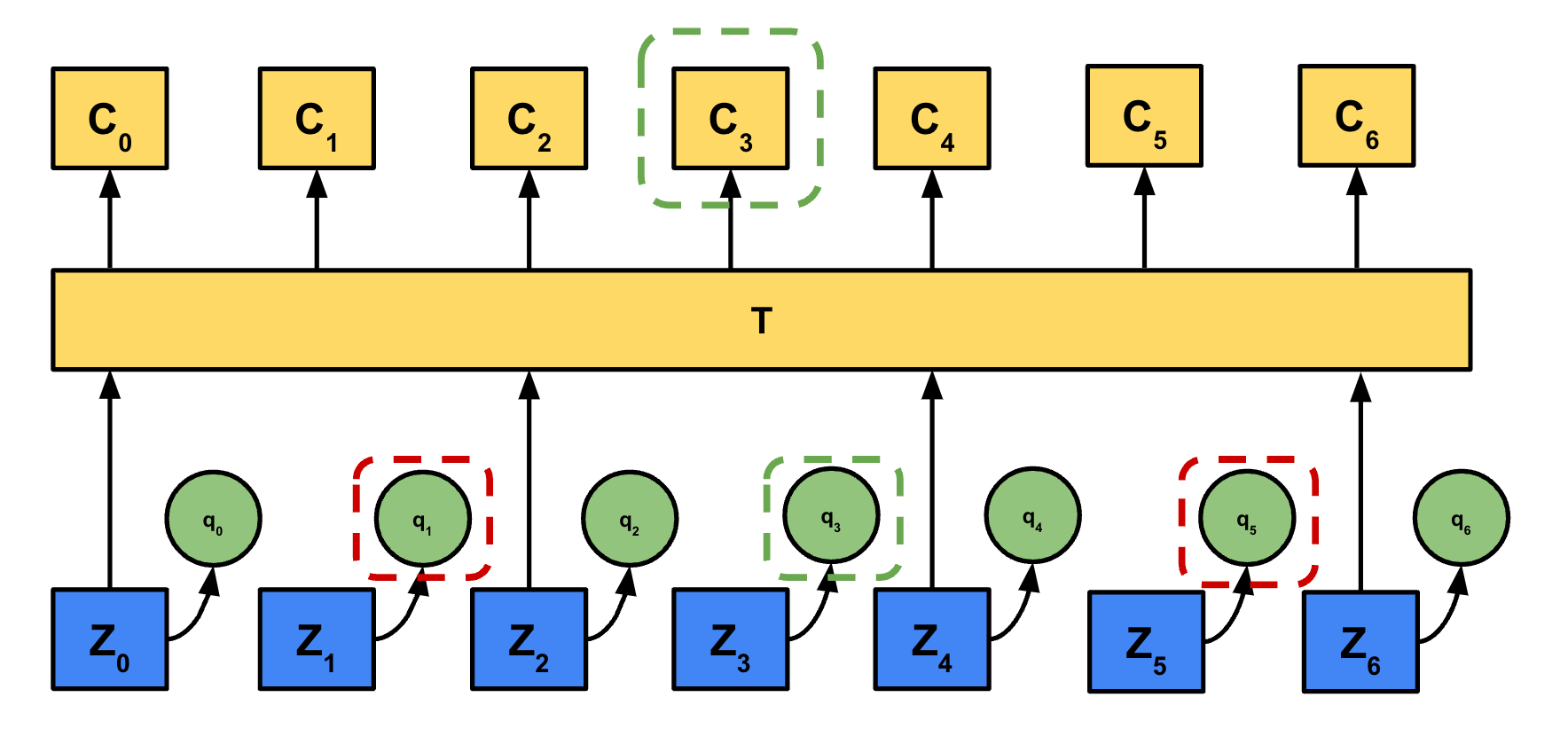
Complete Architectural Diagram

Loss Functions
At this point we have established the architecture but not the loss functions which guides the learned mappings f and g.
Contrastive Loss
The contrastive loss encourages similarity between a candidate vector and target vector and discourages similarity between all other distractor vectors and the target vector. To calculate similarity between two vectors we use the cosine similarity function in eq. 3.
To encourage dissimilarity between the distractor samples we sum their similarity scores in the denominator of the loss function.
For Wav2vec 2.0, we want to match the context representation ct to the quantized representation centered at the same timestep qt, and want to discourage similarity between ct and K distractor quantized representations [qa, …, qb]. Note that qt, and the K distractors [qa, …, qb] all come from masked time steps.
Eq. 4 shows a similarity score we would want to maximize. This function has a maximum value of 1, if sim(ct ,qt) = 1 and all other sim(ct ,q) = 0. Note the denominator is critical: if we only had the numerator, then all q could collapse to the same value and we would still minimize the loss - thus resulting in mode collapse.
The final contrastive loss term used by the authors involves a temperature parameter κ, which we apply in the log domain. Finally, we want to minimize the loss, and so we take the negative of the equation.
Diversity Loss
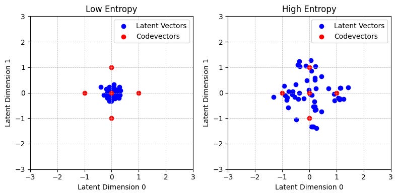
The authors additionally include a diversity loss to encourage the equal use of all the codevectors. In the ‘Low Entropy’ plot above, we can see that most latent vectors map to the codevector centered at (0, 0), whereas on the right the latent vectors are more evenly spread out amongst the 5 codevectors. Recall that this model learns the mapping of the latent vectors and the position of the codevectors jointly, meaning the codevectors are not fixed.
To actually chose which codevector, we compute the similarity score from eq. 3 between our latent z and all the codevectors in a codebook. We use this similarity score as an unnormalized probability value (logit), called l. Therefore we will have one logit per codevector in a given codebook, lg,v. We then apply the below formula to get a probability distribution representing the probability we select codevector v from codebook g for any one latent vector.
During inference, to chose the codevector to represent a particular latent vector we simply select the most probable logit, i.e. codevector index i = argmaxj pg, j.
During training however, we need a differentiable operation to calculate a gradient. To do this, we add noise via the Gumbel softmax term, nv = − log(− log(Uniform(0, 1))). This allows us to treat the discrete argmax operation to chose which logit as a continuous softmax operation and allows the gradient to flow through the softmax. The temperature parameter Tau controls how peaky the distribution is when doing backpropagation.
We can now use eq. 6 above to calculate the entropy which we will use in the diversity loss. Recall that our objective is to have even utilization of all codevectors V. This corresponds to high average entropy, meaning we don’t want all the latent vectors to map to a small set of codevectors, and thus have a high probability mass associated with a small number of codevectors.
Eq. 8 above penalizes the model for having low average entropy across and thus utilize all codevectors. Note our objective is to minimize the loss, and so we introduce a negative sign to penalize low entropy.
Training
Finally, we combine the diversity loss (eq. 8) with the contrastive loss (eq. 5) to give us our overall loss function:
The model is pretrained on a large corpus of speech. For downstream tasks such as speech recognition, the authors add a randomly initialized linear projection layer on top of the context representation, and fine-tune on a smaller dataset.